Linux Scheduling

Process Scheduling In Linux

Introduction

Scheduling is the action of assigning resources to perform _tasks.
We will mainly focus on scheduling where our resource is a processor or multiple processors, and the task will be a thread or a process that needs to be executed.

The act of scheduling is carried out by a process called **scheduler.
**The scheduler goals are to

• Maximize throughput (amount of tasks done per time unit)
• Minimize wait time (amount of time passed since the process was ready until it started to execute)
• Minimize response time (amount of time passed since the process was ready until it finished executing)
• Maximize fairness (distributing resources fairly for each task)

Before getting to the how process scheduling works in Linux, let’s review simpler scheduling algorithms and examples.

Scheduling 101

In case you are familiar with scheduling in general, and don’t need another review of it, go ahead and skip to the next section.

There are two main types of schedulers — Preemptive and non-preemptive schedulers.
If a scheduler is preemptive it might decide at some point that process A had enough CPU for now and decides to hand it to another process.
A non-preemptive scheduler doesn’t support this behavior and CPU is yielded when a process terminates or the process is waiting for some I/O operation and in the meantime is sleeping.

How do we measure schedulers?

There are a few main metrics we will focus on, but before we do, let’s try to give an illustration of what a scheduler might look like

In the above illustration, you can see that our machine has 3 cores.
The numbers indicate the order of arrival.
The first job came and demanded 1 core for 3-time units, then the second one came and demanded 2 cores for 5-time units, and so on.

Utilization

Utilization is defined by the percentage of time that our CPU is busy.
In the case above we have 18 available blocks but only 16 of them are being used, meaning that the utilization here is 0.888 (88.8%).

Throughput

Throughput is defined by how much work is done per time unit.
In our case, 3 processes finish their execution in 6-time units meaning that our throughput is 0.5.

Wait Time

Wait time is defined by the difference between the time the job was submitted and the time it actually started to run.
In our case, job 3 could hypothetically be submitted in time unit 2 but at this point, jobs 1 and 2 took all the resources which made job 3 waits until it had enough resources to start running.

Response Time

Response time is defined by the difference between the time the job was submitted and the termination time.
Assuming job 3 was submitted in time unit 2 and terminated in time unit 6 it means the response time of this job is 4.

Scheduling Algorithms Examples

FCFS - First-Come First-Served

The name is pretty self-explanatory — Jobs are scheduled by their arrival time.
If there are enough free cores, an arriving job will start to run immediately.
Otherwise, it waits until enough cores are freed.

The above diagram illustrates shows how FCFS would work, and we can immediately see that we can optimize it.
As we see, job 4 only requires two cores for a single time unit and it can be scheduled on the unutilized cores.

Pros:

• Easy to implement — FIFO wait queue
• Perceived as most fair

Cons:

• Creates fragmentation — the unutilized cores
• Small or short jobs might wait for a long time

FCSFS With Backfilling

This variation of FCFS reduces the number of unutilized cores.
Whenever a job arrives or terminates, we try to start the head of the wait queue — as we did in the original FCFS.
Then, iterate over the waiting jobs and try to backfill them.

Backfilling happens when a short waiting job can “jump over” the head of the wait queue without delaying its start time.

As you can see, job 3 wasn’t delayed but we could make job 4 jumps over it and execute while job 3 waits for enough resources.

Pros:

• Less fragmentation — better utilization

Cons:

• Must know runtimes in advance in order the calculate the size of the “holes” and to know which candidates can be backfilled.

SJF - Shortest-Job First

Unlike FCFS, instead of ordering jobs by their arrival time, we order time by their estimated runtime.
This algorithm is optimal in the metric of average wait time, let’s try to get some intuition why.

Let’s assume that performing FCFS led us to this point

Let’s try to think how it would be different with SJF and compute the respective average wait time.

Regarding the FCFS scheduler (first illustration):

• job 1 waits 0 time units
• job 2 waits 3 time units
• job 3 waits 4 time units

Hence, the average wait time is (0+3+4)/3 = 7/3

Let’s do the same for the SJF scheduler (second illustration):

• job 1 waits 2 time units
• job 2 waits 0 time units
• job 3 waits 1 time unit

The average wait time, in this case, is (2+0+1)/3 = 1

Process Scheduling In Linux

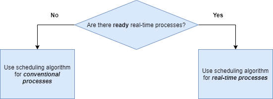
Linux has two types of processes

• Real-time Processes
• Conventional Processes

Real-time processes are required to ‘obey’ response time constraints without any regard to the system’s load.
In different words, real-time processes are urgent and cannot be delayed no matter the circumstances.

An example of a real-time process in Linux is the migration process which is responsible for distributing processes across CPU cores (a.k.a load balancing).

Conventional processes don’t have strict response time constraints and they can suffer from delays in case the system is ‘busy’.

An example of a conventional process can be the browser process you’re using to read this post.

Each process type has a different scheduling algorithm, and as long as there are ready-to-run real-time processes they will run and make the conventional processes wait.

Real-Time Scheduling

There are two scheduling policies when it comes to real-time scheduling, SCHED_RR and SCHED_FIFO.

The policy affects how much runtime a process will get and how is the runqueue is operating.

Since I didn’t mention it explicitly before, let’s get something in order.
The ready-to-run processes I have mentioned are stored in a queue called runqueue. The scheduler is picking processes to run from this runqueue based on the policy.

SCHED_FIFO

As you might have guessed, in this policy the scheduler will choose a process based on the arrival time (FIFO = First In First Out).

A process with a scheduling policy of SCHED_FIFO can ‘give up’ the CPU under a few circumstances:

• Process is waiting, for example for an IO operation.
  When the process is back to ‘ready’ state it will go back to the end of the runqueue.
• Process yielded the CPU, with the system call _sched_yield.
  _The process will immediately go back to the end of the runqueue.

SCHED_RR

RR = Round Robin
In this scheduling policy, every process in the runqueue gets a time slice (quantum) and executes in his turn (based on priority) in a cyclic fashion.

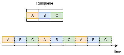
In order for us to have a better intuition about round robin, let’s consider an example where we have 3 processes in our runqueue, A B C, all of them have the policy of SCHED_RR.
As shown in the drawing below, each process gets a time slice and executes in his turn. when all processes ran 1 time, they repeat the same execution order.

Conventional Scheduling

CFS — Completely Fair Scheduler is the scheduling algorithm of conventional processes since version 2.6.23 of Linux.

Remember the metrics of schedulers we discussed at the top of this article? so CFS is focusing mainly on one metric — it wants to be fair as much as possible, meaning that he gives every process gets an even time slice of the CPU.
Note that, processes with higher priority might still get bigger time slices.

In order for us to understand how CFS works, we will have to get familiar with a new term — virtual runtime (vruntime).

Virtual Runtime

Virtual runtime of a process is the amount of time spent by actually executing, not including any form of waiting.

As we mentioned, CFS tries to be as fair as possible.
To accomplish that, CFS will schedule the process with the minimum virtual time that is ready to run.

CFS maintains variables holding the maximum and minimum virtual runtime for reasons we will understand soon.

CFS — Completely Fair Scheduler

Before talking about how the algorithm works, let’s understand what data structure this algorithm is using.

CFS uses a red-black tree which is a balanced binary search tree — meaning that insertion, deletion, and look-up are performed in O(logN) where N is the number of processes.

The key in this tree is the virtual runtime of a process.

New processes or process that got back to the ready state from waiting are inserted into the tree with a key vruntime=min_vruntime.
This is extremely important in order to prevent starvation of older processes in the tree.

Moving on to the algorithm, at first, the algorithm sets itself a time limit — sched_latency.
In this time limit, it will try to execute all ready processes — N.
This means that each process will get a time slice of the time limit divided by the number of processes — Qᵢ = sched_latency/N.

When a process finishes its time-slice (Qᵢ), the algorithm picks the process with the least virtual runtime in the tree to execute next.

Let’s address a situation that might be problematic with the way I described the algorithm so far.
Assuming that the algorithm picked a time limit of 48ms(milliseconds) and we have 6 processes — in this case, every process gets 8ms to execute in his turn.

But what happens when the system is overloaded with processes?
Let’s say the time limit remains 48ms but now we have 32 processes, now each process has 1.5ms to execute — and this will cause a major slowdown in our system.

Why? What’s the difference?

Context switches.
A context switch is a process of storing the state of a process or thread so that it can be restored and resume execution at a later point.

Every time that a process finishes its execution time and a new process is scheduled, a context switch occurs which also takes time.

Let’s say that a context switch costs us 1ms, in the first example where we have 6ms per process, we can allow that, we waste 1ms on the context switch and 5ms on actually executing the process. but in the second example, we only have 0.5ms to execute the process — we waste most of our time slice for context switching and that’s why it simply cannot work.

In order to overcome this situation, we introduce a new variable that will determine how small a time slice is allowed to be — min_granularity.

Let’s say that min_granularity=6ms and get back to our example.
Our time limit is 48 and we have 32 processes.
By the calculation we made before, every process will get 1.5ms but now it is simply not allowed because the min_granularity specifies the minimum time slice each process should get.

In this case, where Qᵢ < min_granularity we take min_granularity as our Qᵢ and change the time limit according to it.

In our example, Qᵢ would be equal to 6ms since 1.5ms < 6ms and that would mean that the new time limit would be Qᵢ ⋅ N = 6ms ⋅ 32 = 192ms.

---

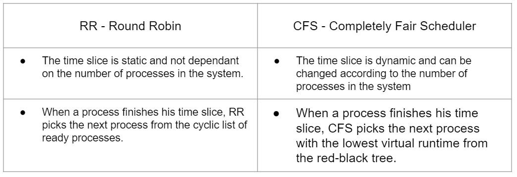
To Summarize, the differences between RR and CFS are as follows